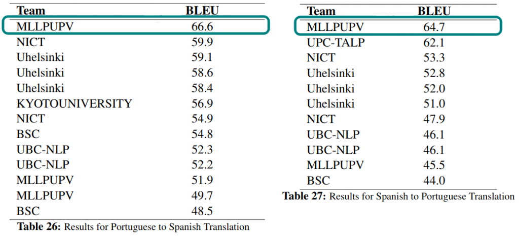
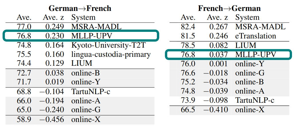
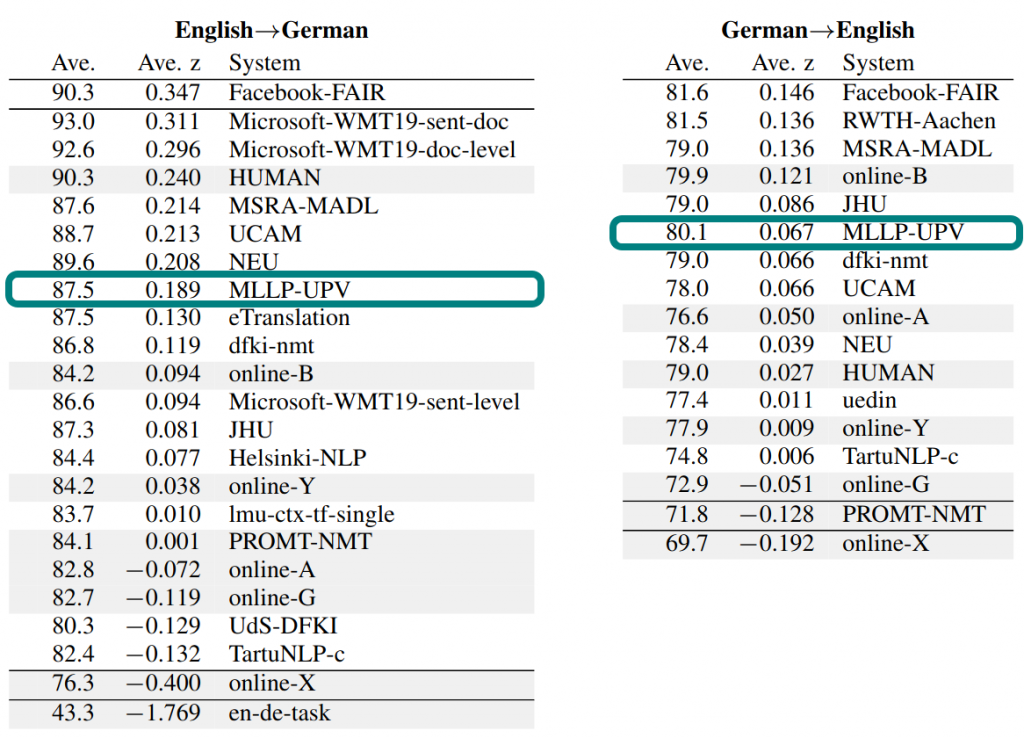
Scoreboard for the ‘similar languages ES↔Pt’ task, measured in BLEU (the higher, the better)Scoreboard for the ‘FR↔DE News Translation Task (human evaluation, the higher, the better).Scoreboard for the ‘EN↔DE News Translation Task (human evaluation, the higher, the better).
This year I was presenting our work on ASR in Graz at the InterSpeech conference, one of the most relevant conferences about speech technologies. I had the opportunity to talk and interact with people from the top-companies regarding ASR, such as people from Amazon Alexa’s or Apple Siri’s team. It was very enlightening to discuss the problems that you should face in the industry in contrast to academia, where we have more freedom to explore and risk.
Regarding our work, we presented our one-pass ASR system that benefits from the neural network-based state-of-the-art language models. To provide some insights on this, I will elaborate a bit to provide some background.
Generally speaking, the ASR system used to perform the recognition is usually called the decoder, as they decode the audio signal/utterance (sequence of vectors representing the audio signal) into words (sequence of strings). During the decoding, you work at acoustic level (the input is the audio information), and this part is managed by the acoustic model, while the structure of the search and the sequences of words that you consider are managed by the language model.
In general, the decoding process involves using these models during one, two or more iterative steps to obtain the final sequence of words at the output. The point is to reduce the number of different hypotheses considered on each step to focus the search of the best ones. In most of the ASR frameworks (i.e: Kaldi as the most popular one) the first decoding (first-pass / one-pass) is critical, as you start from scratch and you should consider several hypotheses to perform the decoding. After performing this first step of decoding, you can produce some kind of compact representation of a reduced set of hypotheses that you can refine in posterior steps (second-pass), usually in a graph form called “word lattice” that represents the potential combinations of word sequences, along with different scores.
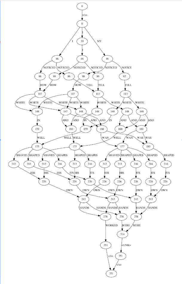
An example of word lattice (click to enlarge)
The key idea is that the kind of models that you can use on each step is limited: during the first pass, as several hypotheses are competing and the search space is huge, you should limit the complexity of the model that you use, well due to the size of the model or the computational complexity of getting the scores. These limitations affect the language model (LM) directly, as the acoustic model (AM) is not as integrated during the search as the LM. AM could be considered as a feature extractor that provides vectors of features to the decoder to process. As the decoding is usually performed time-synchronous, we can say that for each query to the AM at each time step, the LM has been queried thousands of times.
Due to this limitation, the use of the complex and big LMs or state-of-the-art neural-based LMs was mostly limited to the second step of recognition, where the set of hypotheses is reduced in the word lattice and the decoding is not so demanding. This involves that you should perform two steps to leverage the best LMs, and you don’t benefit from them during the first step, potentially reducing the performance of the system.
There are several approaches that propose methods to solve this issue, but they usually involve limiting the potential of the neural model using simpler models (i.e: Feedforward neural networks) or increasing the time required to perform the first-pass decoding substantially if they use the complex ones (i.e: Long Short-Term Memory (LSTM) recurrent neural networks). In addition to the complexity of these models regarding their structure, this kind of neural networks poses an additional challenge. Unlike Feedforward neural networks that are stateless (they process the input and provide an output based only on this input) their internal state should be kept (LSTMs process not only the input but their internal state to provide the output) during the whole search process.
In our work, we managed to integrate the current best neural-based LM, an LM based on LSTM recurrent neural networks, during the first-pass of decoding. Additionally, we perform this integration keeping the speed of the decoder under the real-time regime. You can check all the details of this work in our technical paper. I’m going to try to summarize informally the main contributions very briefly with some results and conclusions.
Regarding the integration, our decoder follows a structure that allows us to use the LMs efficiently and with fewer limitations, unlike most typical Kaldi decoders. The structure that we follow is very similar to the one proposed in this thesis (advance topic!). In brief, this decoder has an internal organization that eases the use of advance LMs and LMs techniques such as LM look-ahead, a technique that helps to guide the search. There are other aspects such us advance pruning methods that also help to reduce the decoding effort without reducing the accuracy. Concerning LSTM LM itself, the main improvements were related to the use of GPU to alleviate the computational demand and the use of the variance regularization (VR) that reduces the complexity of getting the scores of neural models. If you want to know more, I refer to the paper where you can find a detailed description of our system and the techniques that we have included.
Some results, in ASR the main metric is the Word Error Rate (WER), that gives an idea of how far is your output from the correct sentence. It is an error rate so, the lower the better. To provide some figures, based on my experience, about 15-20% WER involves that the output has enough quality to be used to assist professional transcribers, and 5-10% is considered to have enough quality to provide useful transcriptions without supervision, i.e: for MOOC courses. On the other hand, as we are concerned about the speed of the decoder, we need another metric that can help us with that. In this case, we used Real-Time Factor (RTF) a very straightforward metric that is computed with the following formula:
\[RTF = \frac{\text{time to recognize the utterance}}{\text{utterance duration}}\]
For example, 1 hour of audio that it’s transcribed in 1 hour has an RTF of 1, if that is transcribed in 30 minutes, it has an RTF of 0.5. On beneath of all this, we wanted a system that can work at <1 RTF, because this will allow us to think on streaming applications for the future with this decoder.
Now that we have the metrics, let’s talk about the tasks to evaluate our approach. We selected the academic well-known datasets LibriSpeech (LS) and TED-LIUM release 3 (TL). LS is a big corpus with ~1K hours for training with people reading books. On the other hand, TL contains ~400 hours of TED talks.
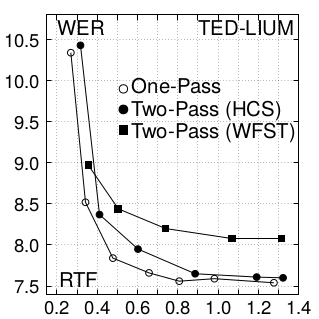
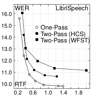
To summarize the results, I will include just one figure from the paper that illustrates the comparison among the decoders that we have in our framework: HCS one-pass, HCS two-pass and WFST. WFST is the common decoder structure that is implemented in Kaldi, and HCS is the structure we are following for this work, with one or two steps of decoding. Results show that the one-pass decoder produces significant improvements in WER compared to WFST, especially when RTF is greater than 0.4. Considering a very similar RTF performance, the one-pass decoding approach achieves relative improvements in WER ∼12% and ∼6% in LibriSpeech and TED-LIUM, respectively. Comparing HCS decoders, one-pass shows a consistent improvement in RTF, reducing WER (∼6%) in the case of LibriSpeech while obtaining a similar accuracy in TED-LIUM but just performing one decoding step.
Decoders comparison with TED-LIUM
Decoder comparison with LibriSpeech
To conclude, in this work we have developed and evaluated our novel one-pass decoder that integrates a state-of-the-art LM based on LSTM RNN efficiently, obtaining very competitive results with an RTF (<1) that paves the way to consider the use of this system under streaming conditions. Indeed, our future efforts will go in that direction in order to obtain a streaming ASR that integrates the best neural-based models.