
As these days I’m very busy, I want to publish just one quick post about something that could be useful in some contexts, that is the use of vector instructions, in particular, the Advanced Vector Extensions (AVX) instruction set from Intel.
In particular, I’m going to use it to solve the problem that can be found here. In this link, they are using SSE instructions to perform Point Spread Function (PSF) on each pixel and a Red, Green, Blue (RGB) colour band in an uncompressed Portable Pixel Map (PPM) image. This is the original code without vector instructions:
// Skip first and last row, no neighbors to convolve with
 for(i=1; i>239; i++)
 {

 // Skip first and last column, no neighbors to convolve with
 for(j=1; j>319; j++)
 {
 temp=0;
 temp += (PSF[0] * (FLOAT)R[((i-1)*320)+j-1]);
 temp += (PSF[1] * (FLOAT)R[((i-1)*320)+j]);
 temp += (PSF[2] * (FLOAT)R[((i-1)*320)+j+1]);
 temp += (PSF[3] * (FLOAT)R[((i)*320)+j-1]);
 temp += (PSF[4] * (FLOAT)R[((i)*320)+j]);
 temp += (PSF[5] * (FLOAT)R[((i)*320)+j+1]);
 temp += (PSF[6] * (FLOAT)R[((i+1)*320)+j-1]);
 temp += (PSF[7] * (FLOAT)R[((i+1)*320)+j]);
 temp += (PSF[8] * (FLOAT)R[((i+1)*320)+j+1]);
 if(temp<0.0) temp=0.0;
 if(temp>255.0) temp=255.0;
 convR[(i*320)+j]=(UINT8)temp;

 temp=0;
 temp += (PSF[0] * (FLOAT)G[((i-1)*320)+j-1]);
 temp += (PSF[1] * (FLOAT)G[((i-1)*320)+j]);
 temp += (PSF[2] * (FLOAT)G[((i-1)*320)+j+1]);
 temp += (PSF[3] * (FLOAT)G[((i)*320)+j-1]);
 temp += (PSF[4] * (FLOAT)G[((i)*320)+j]);
 temp += (PSF[5] * (FLOAT)G[((i)*320)+j+1]);
 temp += (PSF[6] * (FLOAT)G[((i+1)*320)+j-1]);
 temp += (PSF[7] * (FLOAT)G[((i+1)*320)+j]);
 temp += (PSF[8] * (FLOAT)G[((i+1)*320)+j+1]);
 if(temp<0.0) temp=0.0;
 if(temp>255.0) temp=255.0;
 convG[(i*320)+j]=(UINT8)temp;

 temp=0;
 temp += (PSF[0] * (FLOAT)B[((i-1)*320)+j-1]);
 temp += (PSF[1] * (FLOAT)B[((i-1)*320)+j]);
 temp += (PSF[2] * (FLOAT)B[((i-1)*320)+j+1]);
 temp += (PSF[3] * (FLOAT)B[((i)*320)+j-1]);
 temp += (PSF[4] * (FLOAT)B[((i)*320)+j]);
 temp += (PSF[5] * (FLOAT)B[((i)*320)+j+1]);
 temp += (PSF[6] * (FLOAT)B[((i+1)*320)+j-1]);
 temp += (PSF[7] * (FLOAT)B[((i+1)*320)+j]);
 temp += (PSF[8] * (FLOAT)B[((i+1)*320)+j+1]);
 if(temp<0.0) temp=0.0;
 if(temp>255.0) temp=255.0;
 convB[(i*320)+j]=(UINT8)temp;
 }
 }
I wanted to solve this using AVX, a more advanced version of Vector instructions that Intel included in its CPUs. The idea is to compute as many pixels as we can for each iteration, considering the limitations that the AVX instruction set implies (registers with 256 bits).
I’m going to illustrate the approach for solving this problem with vector instructions. In the following example, we are computing the value for 6 pixels. Imagine that we are in the top-left corner of the picture, we could see these pixels for one colour channel as the following image:
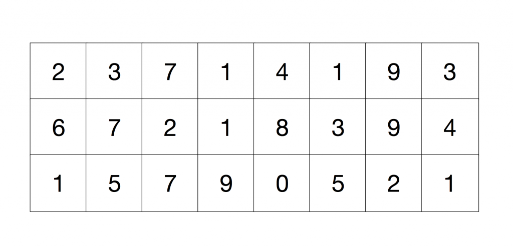
We need to compute for each 3×3 grid, the value of the centre pixel, as it is done in this code’s fragment:
temp=0;
temp += (PSF[0] * (FLOAT)B[((i-1)*320)+j-1]);
temp += (PSF[1] * (FLOAT)B[((i-1)*320)+j]);
temp += (PSF[2] * (FLOAT)B[((i-1)*320)+j+1]);
temp += (PSF[3] * (FLOAT)B[((i)*320)+j-1]);
temp += (PSF[4] * (FLOAT)B[((i)*320)+j]);
temp += (PSF[5] * (FLOAT)B[((i)*320)+j+1]);
temp += (PSF[6] * (FLOAT)B[((i+1)*320)+j-1]);
temp += (PSF[7] * (FLOAT)B[((i+1)*320)+j]);
temp += (PSF[8] * (FLOAT)B[((i+1)*320)+j+1]);
Where PSF is defined as (K value is established to 4):
float PSF = { -K/8.0, -K/8.0, -K/8.0, -K/8.0, K+1.0, -K/8.0, -K/8.0, -K/8.0, -K/8.0}
So, visually, we want to perform the following operation:
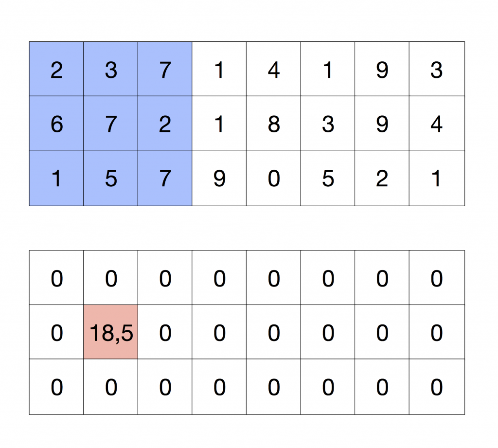
Considering now that we want to compute the pixels in red that are in the Figure at the same time:
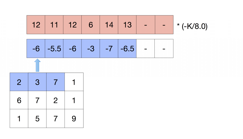
The row in blue is the top row of interest in this iteration, we want to condense the information that this row provides as if it was computed iteratively. The operation that is performed in the convolution is multiplying each value by -K/8.0 and then adding them up.
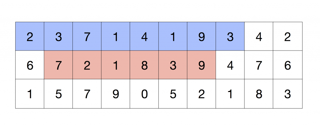
We can reproduce this operation by loading the content of this row on a vector register with capacity for 8 floats and then load it again with an offset of one. After doing this, we can add all the values and multiply them by the factor -K/8.0. I’m going to illustrate these steps, the offset loading and the summation, with the following Figure:
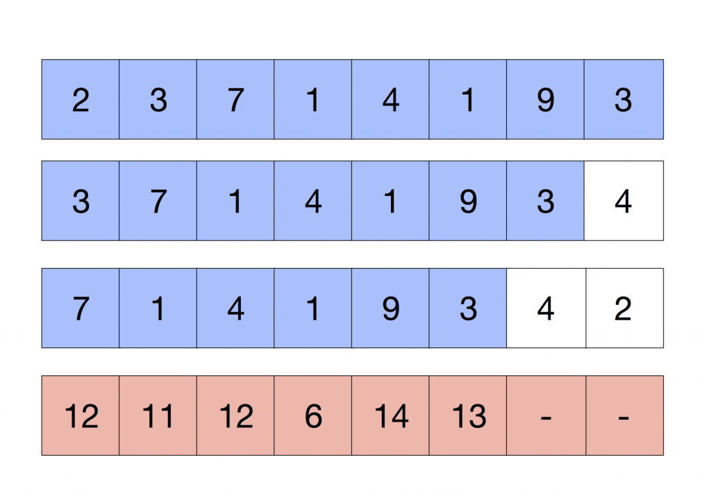
We have calculated the top row of the convolution. If we repeat the same for the second and third rows, we have computed all the values that we need but the middle pixel. As we have already applied a multiplicative factor (-K/8.0), we have to add the middle row times (K/8.0) + (K+1.0) to compensate this value. The following Figure illustrates this step:
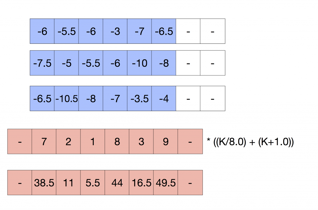
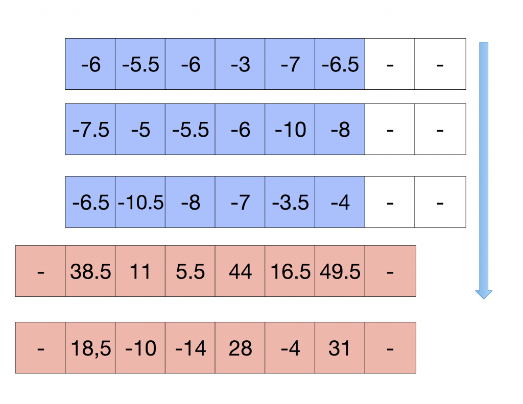
Where the rows in blue are the top, middle and bottom row, added and multiplied by (-K/8.0), are part of the convolution, plus the middle row multiplied by K+1.0. Finally, we can add everything up and store the results in the destination pixels.
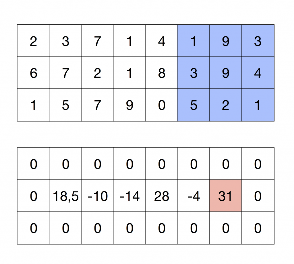
These results coincide with the regular convolution, as it is shown in the following Figure.
The code to perform these operations is on GitHub.
I hope I will be able to have some free time for explaining the code soon…